Offline Reinforcement Learning for Plasma Control in Nuclear Fusion: Codebase and Benchmark

Fu, Yang; Bao, Haomin; Sonker, Rohit; Hu, Xiaoyan; Venugopal, Aravind; Schneider, Jeff; Chen, Jiayu

Agentic Intelligence Lab | HKU

Offline Reinforcement Learning for Plasma Control in Nuclear Fusion

Yang Fu^*,1, Haomin Bao^*,1, Rohit Sonker², Xiaoyan Hu², Aravind Venugopal², Jeff Schneider², Jiayu Chen^†,1

¹The University of Hong Kong, ²Carnegie Mellon University

^*Indicates equal contribution. ^†Indicates corresponding author.

NeurIPS 2026

Paper arXiv Code Dataset Quick Tutorial BibTeX

Abstract

Offline reinforcement learning (RL) offers a promising route for developing plasma controllers from historical tokamak data, since online trial-and-error on real devices is costly and risky. However, progress in this direction remains difficult to measure due to the lack of a standardized offline RL benchmark for realistic multi-actuator, long-horizon plasma control problems in nuclear fusion. We introduce RL4F, an Offline Reinforcement Learning Benchmark for Plasma Control in Nuclear Fusion, providing closed-loop evaluation environments and baseline comparisons across four full-profile tracking tasks: rotation, density, temperature, and pressure. The dynamics function underlying the evaluation environment is built from historical discharge data from DIII-D, a real-world tokamak. We evaluate a broad set of imitation learning and offline RL baselines under a unified protocol. We find that offline model-based RL methods obtain the best average performance on most objectives, although no single method dominates all tasks, highlighting the importance of dynamics modeling in complex, long-horizon plasma control tasks. To foster further research, we open-source the codebase, datasets, and evaluation framework, providing a benchmark not only for the fusion community but also for algorithm development in offline RL. We evaluate a broad set of imitation learning and offline RL baselines under a unified protocol. We find that offline model-based RL methods obtain the best average performance on most objectives, although no single method dominates all tasks, highlighting the importance of dynamics modeling in complex, long-horizon plasma control tasks. To foster further research, we open-source the codebase, datasets, and evaluation framework, providing a benchmark not only for the fusion community but also for algorithm development in offline RL.

Simulator

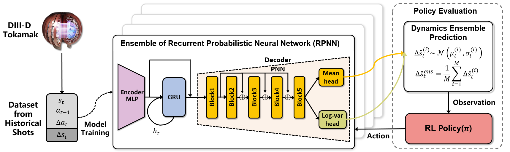
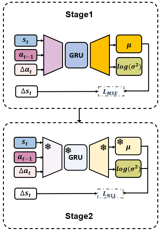
RL4F benchmark workflow with DIII-D data, RPNN dynamics ensemble, and closed-loop policy evaluation

Given the limited accessibility of real tokamak devices, we train a reference dynamics model as a digital twin. The reference dynamics model is trained from historical DIII-D experimental discharges and is used to generate offline training data and to provide the closed-loop evaluation environment. As shown below, we adopt a two-stage RPNN training procedure.

1

Stage 1 Mean Optimization

The first stage optimizes the predictive mean using a mean-squared error objective.

2

Stage 2 Uncertainty Calibration

The second stage initializes from the first-stage checkpoint, freezes the predictive backbone, and trains the log-variance head using a negative log-likelihood objective, thereby calibrating uncertainty without changing the learned mean dynamics.

Two-stage RPNN training procedure with mean prediction and uncertainty calibration

Results

Profile tracking error (RMSE ↓) across radial locations. Values are reported as mean ± standard error over test shots; lower is better.

Table 1: Rotation profile tracking error (RMSE ↓).
Algorithm	ψ_0.06		ψ_0.15		ψ_0.36		ψ_0.55		ψ_0.76		ψ_0.85		Average
Algorithm	Mean	SE	Mean	SE	Mean	SE	Mean	SE	Mean	SE	Mean	SE	Mean	SE
GCIL	32.45	0.376	28.46	0.336	20.73	0.240	15.72	0.180	11.76	0.135	10.28	0.116	17.76	0.047
TD3BC	25.10	0.318	20.99	0.274	14.81	0.189	11.35	0.141	8.69	0.104	7.79	0.092	13.13	0.038
CQL	24.88	0.364	21.09	0.319	15.48	0.241	12.13	0.192	9.28	0.143	8.23	0.120	13.58	0.044
IQL	29.64	0.439	25.72	0.391	18.85	0.275	14.47	0.203	10.87	0.149	9.48	0.129	16.23	0.051
EDAC	26.30	0.427	20.78	0.359	14.43	0.261	11.41	0.210	9.10	0.157	8.31	0.129	13.30	0.048
MCQ	28.45	0.344	24.08	0.310	17.19	0.224	13.22	0.167	10.10	0.120	8.90	0.102	15.10	0.043
PPO	13.96	0.159	10.41	0.138	9.81	0.120	9.85	0.124	8.51	0.112	7.79	0.103	9.36	0.023
COMBO	17.67	0.309	12.85	0.252	8.02	0.160	6.29	0.118	5.29	0.085	5.43	0.074	8.09	0.032
MOPO	18.21	0.241	13.47	0.213	9.19	0.163	7.32	0.130	5.62	0.093	5.20	0.076	8.66	0.030
MOBILE	48.07	0.729	41.59	0.620	30.98	0.438	24.50	0.338	18.93	0.258	16.37	0.221	26.86	0.083
RAMBO	17.22	0.280	12.17	0.216	7.56	0.139	6.33	0.106	5.73	0.082	5.93	0.078	8.03	0.029
BAMCTS	43.47	0.488	38.65	0.433	28.92	0.318	22.24	0.244	16.28	0.181	13.69	0.157	24.38	0.063

Table 2: Density profile tracking error (RMSE ↓).
Algorithm	ψ_0.06		ψ_0.15		ψ_0.36		ψ_0.55		ψ_0.76		ψ_0.85		Average
Algorithm	Mean	SE	Mean	SE	Mean	SE	Mean	SE	Mean	SE	Mean	SE	Mean	SE
GCIL	1.120	0.0135	1.031	0.0128	0.920	0.0121	0.864	0.0117	0.792	0.0115	0.760	0.0113	0.860	0.0021
TD3BC	1.093	0.0132	1.009	0.0126	0.900	0.0117	0.840	0.0113	0.761	0.0109	0.727	0.0107	0.836	0.0021
CQL	1.127	0.0140	1.033	0.0132	0.922	0.0123	0.868	0.0120	0.807	0.0120	0.775	0.012	0.865	0.0022
IQL	1.088	0.0130	0.998	0.0124	0.885	0.0118	0.830	0.0117	0.768	0.0117	0.738	0.0116	0.831	0.0021
EDAC	1.281	0.0157	1.197	0.0151	1.099	0.0144	1.051	0.0142	0.998	0.0145	0.969	0.0145	1.037	0.0026
MCQ	1.059	0.0119	0.983	0.0115	0.891	0.0109	0.840	0.0106	0.768	0.0104	0.735	0.0102	0.828	0.0019
PPO	1.048	0.0131	0.914	0.0125	0.770	0.0115	0.717	0.0108	0.661	0.0100	0.630	0.0096	0.733	0.0020
COMBO	0.966	0.0115	0.870	0.0107	0.745	0.0098	0.676	0.0094	0.602	0.0091	0.578	0.0088	0.691	0.0017
MOPO	0.988	0.0108	0.898	0.0105	0.784	0.0103	0.723	0.0102	0.648	0.0096	0.621	0.0093	0.727	0.0018
MOBILE	1.325	0.0144	1.273	0.0139	1.225	0.0135	1.206	0.0137	1.195	0.0143	1.197	0.0145	1.184	0.0025
RAMBO	1.576	0.0147	1.596	0.0138	1.671	0.0132	1.699	0.0127	1.638	0.0115	1.600	0.0109	1.583	0.0024
BAMCTS	1.220	0.0143	1.165	0.0142	1.101	0.0139	1.058	0.0135	0.975	0.0128	0.938	0.0125	1.023	0.0024

Table 3: Temperature profile tracking error (RMSE ↓).
Algorithm	ψ_0.06		ψ_0.15		ψ_0.36		ψ_0.55		ψ_0.76		ψ_0.85		Average
Algorithm	Mean	SE	Mean	SE	Mean	SE	Mean	SE	Mean	SE	Mean	SE	Mean	SE
GCIL	0.492	0.0055	0.461	0.0052	0.393	0.0045	0.325	0.0037	0.238	0.0028	0.206	0.0025	0.323	0.0008
TD3BC	0.468	0.0051	0.429	0.0047	0.360	0.0039	0.298	0.0033	0.223	0.0026	0.195	0.0024	0.301	0.0007
CQL	0.563	0.0054	0.526	0.0049	0.443	0.0041	0.360	0.0034	0.259	0.0026	0.223	0.0023	0.362	0.0008
IQL	0.465	0.0052	0.429	0.0049	0.362	0.0041	0.301	0.0034	0.225	0.0027	0.196	0.0025	0.302	0.0007
EDAC	0.735	0.0076	0.709	0.0070	0.624	0.0061	0.518	0.0053	0.376	0.0043	0.330	0.0041	0.507	0.0011
MCQ	0.382	0.0046	0.349	0.0043	0.293	0.0037	0.241	0.0030	0.178	0.0023	0.157	0.0021	0.244	0.0006
PPO	0.444	0.0040	0.362	0.0034	0.245	0.0029	0.204	0.0026	0.187	0.0025	0.179	0.0026	0.240	0.0006
COMBO	0.408	0.0038	0.371	0.0035	0.310	0.0030	0.261	0.0026	0.203	0.0022	0.180	0.0021	0.264	0.0006
MOPO	0.276	0.0032	0.246	0.0031	0.212	0.0030	0.190	0.0030	0.163	0.0030	0.156	0.0030	0.193	0.0005
MOBILE	0.623	0.0066	0.580	0.0062	0.488	0.0054	0.403	0.0044	0.304	0.0033	0.273	0.0030	0.408	0.0009
RAMBO	1.044	0.0105	1.004	0.0100	0.848	0.0087	0.652	0.0071	0.406	0.0048	0.332	0.0041	0.655	0.0016
BAMCTS	0.814	0.0115	0.770	0.0107	0.658	0.0089	0.537	0.0072	0.383	0.0052	0.330	0.0046	0.534	0.0015

Table 4: Pressure profile tracking error (RMSE ↓).
Algorithm	ψ_0.06		ψ_0.15		ψ_0.36		ψ_0.55		ψ_0.76		ψ_0.85		Average
Algorithm	Mean	SE	Mean	SE	Mean	SE	Mean	SE	Mean	SE	Mean	SE	Mean	SE
GCIL	17346.5	177.2	15502.4	160.0	10897.1	129.6	8174.0	103.5	4943.7	64.2	3300.2	42.8	8775.3	25.4
TD3BC	15496.3	154.0	13049.8	133.2	9079.8	108.5	6998.2	92.6	4558.2	61.6	3138.1	42.1	7628.9	21.8
CQL	13685.7	144.8	11030.1	123.6	6921.7	92.8	5275.7	74.2	3614.5	48.4	2544.5	33.1	6162.2	19.1
IQL	15518.4	171.7	13089.6	153.7	9041.5	126.1	6788.6	104.7	4312.7	66.9	2951.4	45.0	7525.8	23.8
EDAC	12405.6	139.3	9868.5	114.9	6624.9	81.4	5648.2	68.9	4114.2	48.9	2922.3	34.4	6016.8	17.2
MCQ	14885.6	149.0	12482.0	129.0	8536.6	101.2	6457.9	83.5	4155.5	54.1	2852.5	36.8	7174.3	20.8
PPO	14511.3	143.5	11680.0	117.8	7149.0	80.1	5178.8	63.5	3511.9	41.1	2482.2	28.2	6333.2	18.8
COMBO	14014.7	135.6	11379.7	110.5	7002.4	73.7	4959.2	56.6	3215.5	36.8	2242.7	25.5	6095.9	18.0
MOPO	12706.3	131.5	9894.5	105.4	5534.0	66.7	3997.4	52.9	2892.6	37.4	2094.5	26.5	5198.6	16.5
MOBILE	15342.5	150.7	12692.0	125.8	8178.6	90.7	5738.4	75.3	3464.5	51.9	2353.1	36.1	6854.9	20.7
RAMBO	12437.8	133.2	9786.2	109.9	5790.4	77.2	4391.8	63.4	3171.1	43.2	2276.1	30.0	5358.2	17.0
BAMCTS	18697.5	180.6	16093.4	152.6	11559.1	119.0	8715.9	103.0	5420.3	69.6	3673.5	47.7	9411.5	25.6

Table 5: Q profile tracking error (RMSE ↓).
Algorithm	ψ_0.06		ψ_0.15		ψ_0.36		ψ_0.55		ψ_0.76		ψ_0.85		Average
Algorithm	Mean	SE	Mean	SE	Mean	SE	Mean	SE	Mean	SE	Mean	SE	Mean	SE
GCIL	0.1651	0.0018	0.1429	0.0016	0.0925	0.0010	0.0553	0.0006	0.0245	0.0003	0.0194	0.0002	0.0723	0.0002
TD3BC	0.1455	0.0016	0.1263	0.0014	0.0829	0.0009	0.0557	0.0006	0.0243	0.0003	0.0197	0.0002	0.0652	0.0002
CQL	0.1617	0.0017	0.1399	0.0014	0.0904	0.0009	0.0541	0.0005	0.0250	0.0003	0.0193	0.0002	0.0712	0.0002
IQL	0.1662	0.0020	0.1437	0.0017	0.0928	0.0011	0.0552	0.0006	0.0241	0.0003	0.0191	0.0002	0.0724	0.0002
EDAC	0.1758	0.0018	0.1513	0.0015	0.0961	0.0010	0.0563	0.0006	0.0261	0.0003	0.0224	0.0002	0.0763	0.0002
MCQ	0.1872	0.0022	0.1617	0.0019	0.1038	0.0012	0.0609	0.0007	0.0251	0.0003	0.0195	0.0002	0.0805	0.0003
PPO	0.1407	0.0017	0.1223	0.0015	0.0812	0.0010	0.0519	0.0007	0.0291	0.0004	0.0235	0.0003	0.0658	0.0002
COMBO	0.1159	0.0017	0.1016	0.0015	0.0693	0.0010	0.0458	0.0007	0.0270	0.0004	0.0234	0.0003	0.0562	0.0002
MOPO	0.1151	0.0018	0.1010	0.0016	0.0694	0.0011	0.0500	0.0008	0.0298	0.0004	0.0238	0.0003	0.0564	0.0002
MOBILE	0.1666	0.0019	0.1480	0.0017	0.1062	0.0012	0.0753	0.0008	0.0480	0.0005	0.0419	0.0005	0.0871	0.0002
RAMBO	0.1734	0.0019	0.1505	0.0016	0.0987	0.0011	0.0608	0.0007	0.0300	0.0004	0.0248	0.0003	0.0781	0.0002
BAMCTS	0.1588	0.0018	0.1386	0.0015	0.0928	0.0010	0.0585	0.0007	0.0287	0.0003	0.0229	0.0003	0.0728	0.0002

Table 6: β_N tracking error (RMSE ↓).
Algorithm	Mean	SE
GCIL	0.4145	0.0044
TD3BC	0.3641	0.0032
CQL	0.3336	0.0033
IQL	0.3139	0.0039
EDAC	0.2785	0.0028
MCQ	0.3001	0.0035
PPO	0.2849	0.0026
COMBO	0.2531	0.0025
MOPO	0.2399	0.0028
MOBILE	0.2660	0.0027
RAMBO	0.2041	0.0025
BAMCTS	0.4539	0.0036

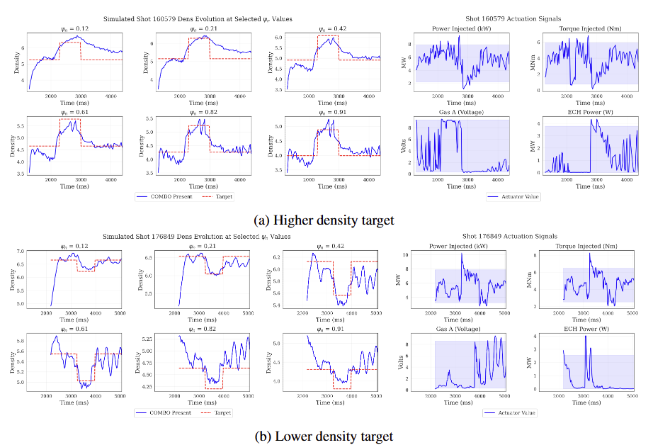
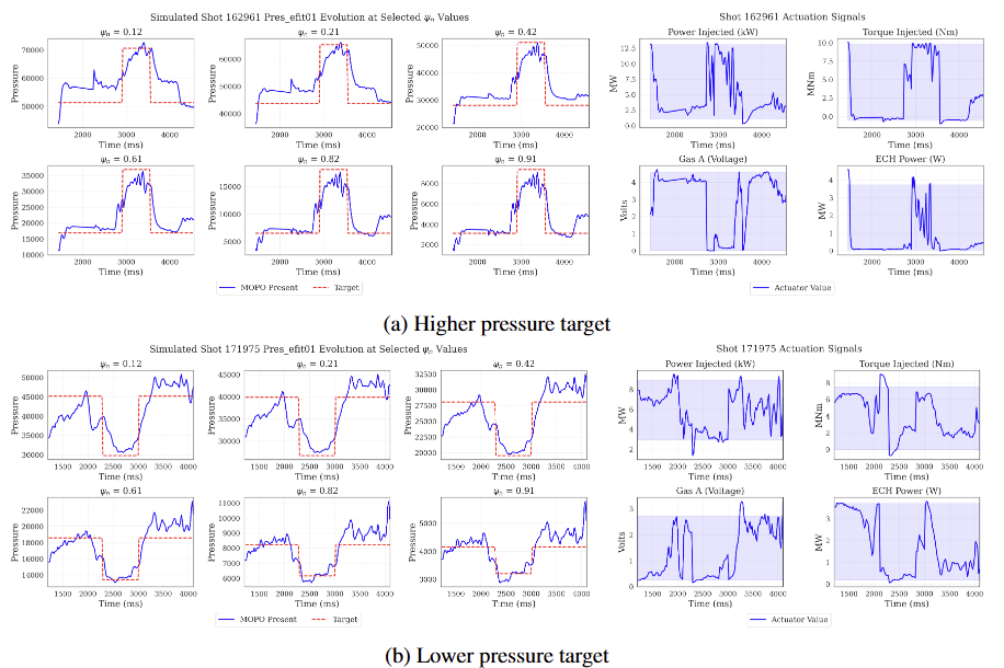
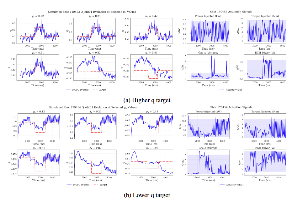
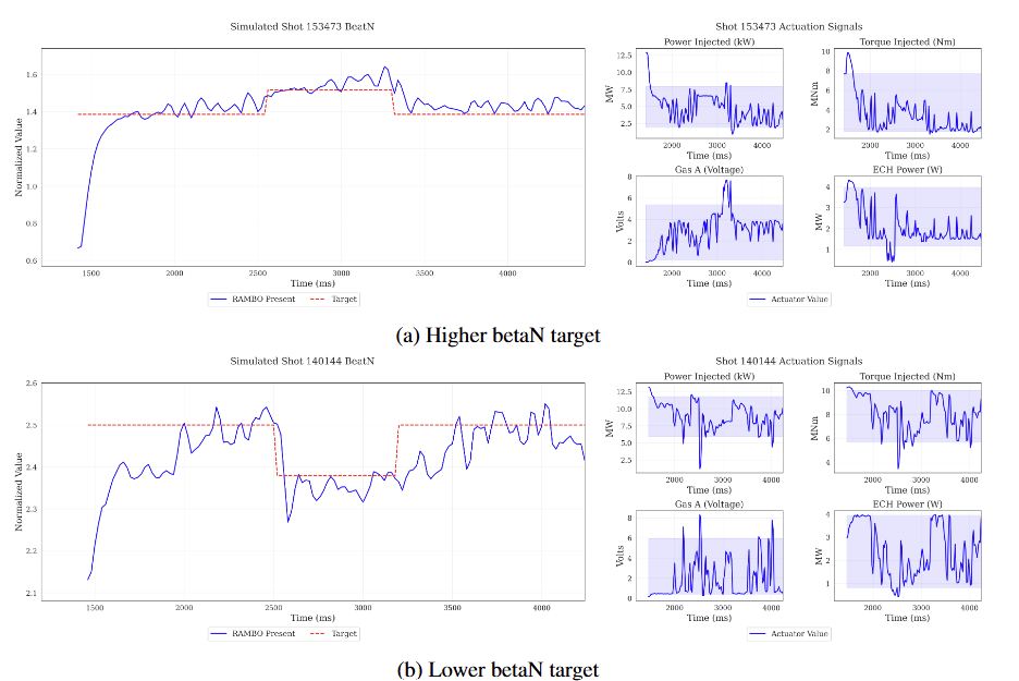
Visualisation Results

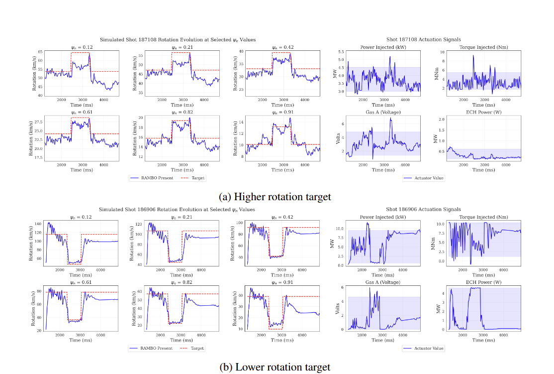
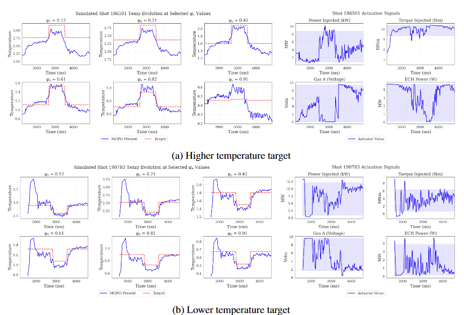
Closed-loop tracking rollouts with actuator signals shown side by side.

Temperature visualisation results showing higher and lower target rollouts alongside actuation signals — **Temperature control examples**Higher and lower temperature-target cases are displayed together with power, torque, gas, and ECH actuator signals. 2 / 6

Density visualisation results showing higher and lower target rollouts alongside actuation signals — **Density control examples**Higher and lower density-target cases are shown with the associated multi-actuator trajectories. 3 / 6

Pressure visualisation results showing higher and lower target rollouts alongside actuation signals — **Pressure control examples**Higher and lower pressure-target cases are paired with the corresponding actuator responses. 4 / 6

q visualisation results showing higher and lower target rollouts alongside actuation signals — **q control examples**Higher and lower q-target cases illustrate closed-loop tracking behavior and actuator usage. 5 / 6

betaN visualisation results showing higher and lower target rollouts alongside actuation signals — **betaN control examples**Higher and lower betaN-target cases are displayed with the matching actuator trajectories. 6 / 6

Quick Tutorial

Set up RL4F, train a controller, and inspect its tracking performance.

Follow the steps below from the source checkout. For the full configuration and API reference, see the repository README.

Install the environment

Clone the repository and create the Conda environment. These commands follow the README's PyTorch 2.1.0 / CUDA 11.8 setup.

git clone --branch release_v1 https://github.com/LucasCJYSDL/Offline-RL-Kit-for-Nuclear-Fusion.git
cd Offline-RL-Kit-for-Nuclear-Fusion
conda env create -f environment.yml
conda activate offline-rl-fusion
pip install torch==2.1.0 torchvision==0.16.0 torchaudio==2.1.0 \
  --index-url https://download.pytorch.org/whl/cu118
pip install -e .

Install the dynamics dependency, then return to the RL4F source checkout:

git clone https://github.com/IanChar/dynamics-toolbox.git
cd dynamics-toolbox
git checkout rohit-tm
pip install -e .
cd ..

Prepare the data and models

Download and extract the processed datasets into data/processed/. Place the pre-trained dynamics models in models/train/ and models/val/.

Download datasets Download dynamics models
Expected directory layout
```
Offline-RL-Kit-for-Nuclear-Fusion/
├── data/
│   └── processed/
│       ├── full.hdf5
│       ├── il_data.h5
│       ├── info.pkl
│       ├── rl_data.h5
│       ├── tracking_test.h5
│       ├── tracking_val.h5
│       └── used_shots_info.txt
└── models/
    ├── train/
    │   ├── 0/
    │   ├── 1/
    │   └── …
    └── val/
```
Using custom data or model locations

Set the relevant environment variables before training: OFFLINERLKIT_DATA_ROOT, OFFLINERLKIT_RAW_DATA_DIR, OFFLINERLKIT_PROCESSED_DATA_DIR, OFFLINERLKIT_MODEL_ROOT, OFFLINERLKIT_TRAINING_MODEL_DIR, and OFFLINERLKIT_EVALUATION_MODEL_DIR.
Train a policy

Start with the README's temperature-control example:
```
python scripts/run_ppo.py --env profile_control_new --task temp
```
Choose a task matching your data: temp, rotation, dens, pres, q, or betan. Other training entry points include run_cql.py, run_iql.py, run_edac.py, run_td3bc.py, run_combo.py, run_mobile.py, and run_mopo.py.

Each script loads its task and algorithm defaults from offlinerlkit/configs/benchmark_configs.json; command-line flags override these defaults. Return plots and policy checkpoints are saved in logs/.
Goal-conditioned imitation learning example
```
python scripts/run_gcil.py --env profile_control --task rotation
```
Evaluate and visualize tracking

Replace /path/to/your_run_dir with your trained policy's run directory. The visualization script detects the algorithm and saves actuator choices, profile-tracking outputs, and tracking-error summaries.
```
python -m visualization.profile_tracking_save --actor_path /path/to/your_run_dir
```
Add --test to evaluate on the test split:
```
python -m visualization.profile_tracking_save --actor_path /path/to/your_run_dir --test
```
Results are written to results/<task>/<algo>/<val|test>/<run>/<seed>/.

Optional: train your own dynamics models

Update data_path and save_path in dynamics/cfgs/rpnn_noshape_gas_benchmark1.yaml and rpnn_noshape_gas_benchmark2.yaml. Before stage two, set its model.load_dir to the model directory produced by stage one.

python dynamics/launch_dynamics.py --cn rpnn_noshape_gas_benchmark1
python dynamics/launch_dynamics.py --cn rpnn_noshape_gas_benchmark2

Evaluate the resulting model:

python dynamics/reevaluate_dynamics.py --model_dir /path/to/trained_model

Q&A

Join our Slack community to ask questions about RL4F, get help with setup and usage, and discuss the benchmark with other researchers.

https://join.slack.com/t/rl4f/shared_invite/zt-4dejdwwbn-Sb41w_zQZ5dQV8j~MD8abA

BibTeX

@misc{fu2026offline,
  title={Offline Reinforcement Learning for Plasma Control in Nuclear Fusion: Codebase and Benchmark},
  author={Fu, Yang and Bao, Haomin and Sonker, Rohit and Hu, Xiaoyan and Venugopal, Aravind and Schneider, Jeff and Chen, Jiayu},
  year={2026},
  eprint={2606.07550},
  archivePrefix={arXiv},
  primaryClass={cs.LG},
  url={https://arxiv.org/abs/2606.07550}
}

Offline Reinforcement Learning for Plasma Control in Nuclear Fusion

Abstract

Simulator

Stage 1 Mean Optimization

Stage 2 Uncertainty Calibration

Results

Visualisation Results

Quick Tutorial

1Install the environment

2Prepare the data and models

3Train a policy

4Evaluate and visualize tracking

Q&A

BibTeX

Install the environment

Prepare the data and models

Train a policy

Evaluate and visualize tracking